Detection of differentially expressed genes using RNA-Seq
Introduction
In this tutorial we will analyze an RNA-Seq data set to detect differences in gene expression between two experimental conditions. We will use a program called Tophat to align the RNA-Seq reads to the reference genome and a second program called cuffdiff to calculate RPKM (FPKM) and perform a test to detect significantly significant differences between the two conditions.
Requirements
- An account on CyVerse Discovery Environment
- A spreadsheet program (Microsoft Excel or LibreOffice)
- You should have already completed the Getting Started With Discovery Environment tutorial
The data
The sequence reads that we will use in this tutorial are from an experiment published by O’Connell et al 2012. In this experiment the authors monitored gene expression of both a pathogen and its host plant during the infection process at several time points. For this tutorial, we will compare the gene expression of the fungal pathogen at two of the time points: 24 hpi (hours post inoculation) and 60 hpi.
The data that will be used in this tutorial consist of the following:
- The genome sequence of Colletotrichum graminicola. File name: colletotrichum_graminicola_m1.001_1_supercontigs.fasta. The genome sequence consists of 653 supercontigs.
- Gene annotations for Colletotrichum graminicola. File name: cgram.gtf
- Four sets of RNA-Seq reads. Two from the 24hpi time point (2 repetitions) and two from the 60 hour time point (2 repetitions). These files are in FASTQ format.
O’Connell RJ, Thon MR, Hacquard S, Ver Loren Van Themaat E, Amyotte S, Kleemann J, Torres-Quintero M, Damm U, Buite E, Epstein, L., M., Alkan N, Altmüller J, Alvarado-Balderrama L, Bauser C, Becker C, Birren BW, Chen Z, Crouch JA, Duvick J, Farman M, Gan P, Heiman D, Henrissat B, Howard RJ, Kabbage M, Koch C, Kubo Y, Law A, Lebrun MH, Lee YH, et al.: Life-style transitions in plant pathogenic Colletotrichum fungi defined by genome and transcriptome analyses. Nature Genetics 2012, 44:1060–1065
Step 1: Align the reads to the reference genome using tophat.
First, we need to locate the data that we will use in the analysis. Because the data files are so large, I have already uploaded them to Discovery Environment.
Log in to Discovery Environment.
To find the data files, click on the orange Data button. Click on the ‘Shared with me’ folder and then look a folder called mthon. Click on mthon and you should find a folder called rna-seq-tutorial.

Here you will see the four files of sequence reads in FASTQ format as well as the reference genome sequence and the gene annotations.
Now we will align the sequence reads to the reference genome using the program tophat. The gene annotations will be used by tophat to identify the locations of each gene in the genome and to calculate the length of each gene, which is needed to calculate RPKM values.
Click on the orange Apps button.
Search for an app called TopHat2-SE
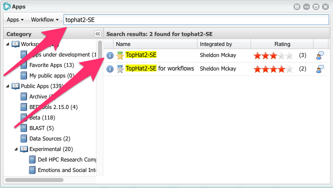
When you find it, click in the app name (TopHat2-SE) to open it.

We will use this window to configure the app and run it. Notice that the app window is divided into 7 sections.
Click on Input data to open this part of the app configuration.
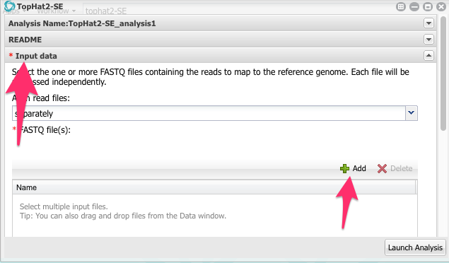
Now, click on the green Add button. Navigate to the folder with the FASTQ files and select all four files:
Click OK.
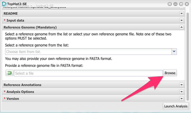
Now we are back in the App configuration window. Scroll down and and click on the section called Reference Genome. Click on it to open it.
Click on the Browse button and then navigate to the Colletotrichum genome sequence and select it.
Open the Reference Annotations section and select the cgram.gtf file.
We’re almost done configuring the app but we still have one more change to make. Open the Analysis Options section and look for two options. On is called Maximum intron length: and the other is called Maximum intron length that may be found during split-segment (default) search:
Change both values to 1000. Remember that the RNA-Seq reads are sequences of fragments of mRNA. mRNA is spliced so it does not contain introns. However, we are aligning the sequences to the genomic sequence which contains the introns. The default value of 500000 may be fine for the human genome but fungal introns are rarely longer than a few hundred bases.
Now the app is configured. Click Launch Analysis.
Open the Analyses list by clicking on the orange Analyses button. The status of your tophat analysis should be Running. The tophat analysis will take a few hours. You can check the status of the analysis by clicking on the refresh button in the Analysis window.
Step 2: Find differentially expressed genes with cuffdiff.
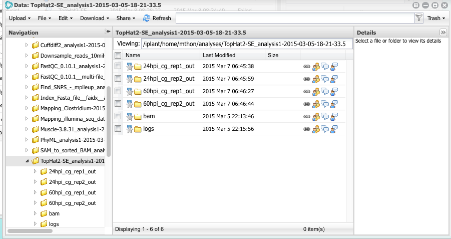
When the analysis is completed you can click on the analysis name to open a Data window showing the results. You will see four folders, one for each FASTQ file that was aligned to the reference genome.
Open the folder named 24hpi_cg_rep1_out. Inside you will see several files. One is names align_summary.txt. click on that file to open it. You will see a report that says of the 25 million sequence reads, 1.8% of them were mapped (aligned) to the reference. Why so few? To understand why, you have to remember the design of this experiment. The RNA samples were taken from maize leaves infected with Colletotrichum graminicola. This particular sample was taken 24 hours after inoculating the leaf. There is very little fungal biomass in the leaves after only 24 hours of inoculation. Open the report for the 60 hpi samples. What percentage of reads mapped to the genome?
Close the report files and return to the folder 24hpi_cg_rep1_out. You will see several other files that were produced by tophat. The most important one is called accepted_hits.bam. This file contains the pairwise alignments of all the reads to the reference genome. These are the files that we will analyze using cuffdiff to compute the FPKM values and perform statistical tests.
All four accepted_hits.bam files have the same name. Before running cuffdiff, let’s rename them. Select the file, then, from the menu, select Edit -> Rename.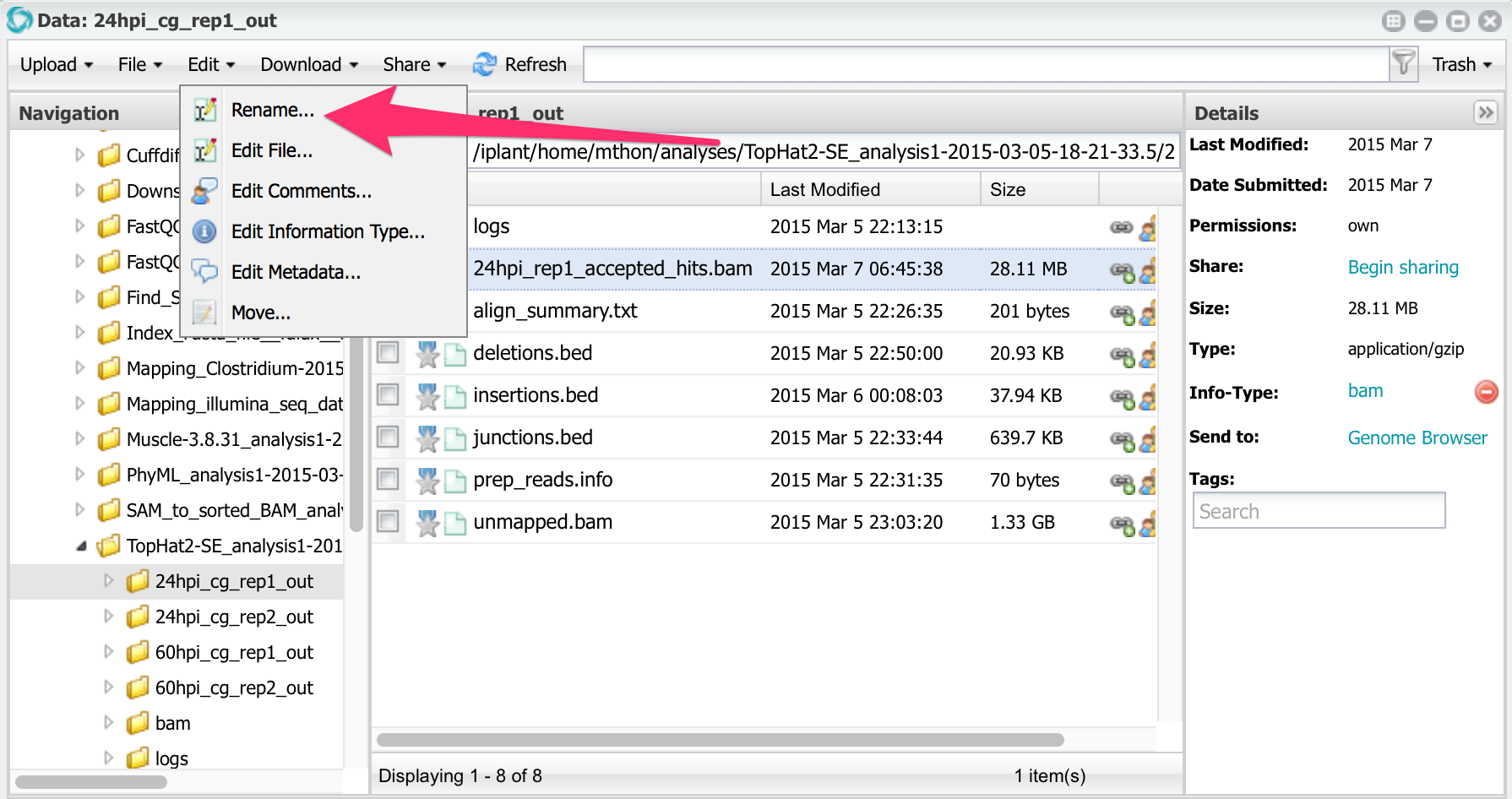 Rename all four files changing the names to this:
24hpi_rep1_accepted_hits.bam
24hpi_rep2_accepted_hits.bam
60hpi_rep1_accepted_hits.bam
60hpi_rep2_accepted_hits.bam
Now we can run cuffdiff. Open the apps window and search for an app named cuffdiff2:
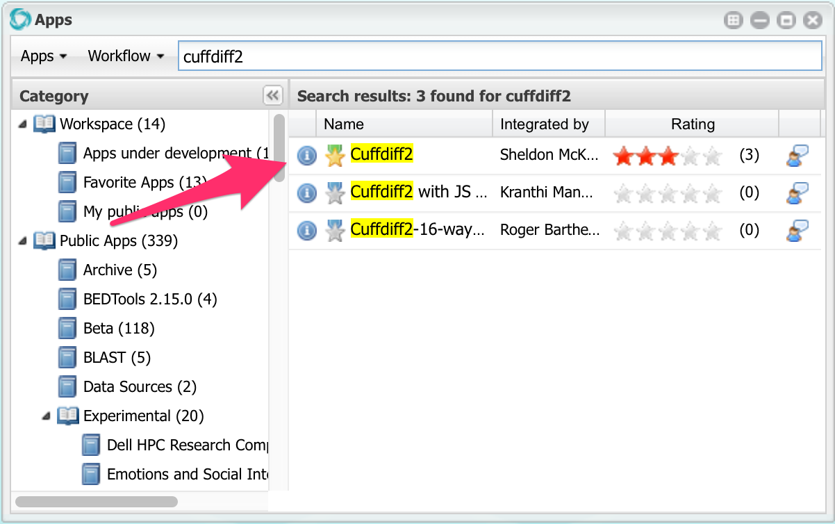
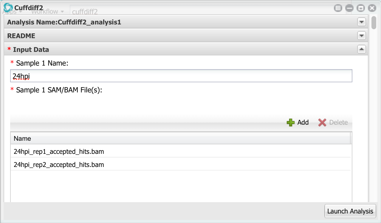
Click on Cuffdiff2 to open it, then click on Input Data:
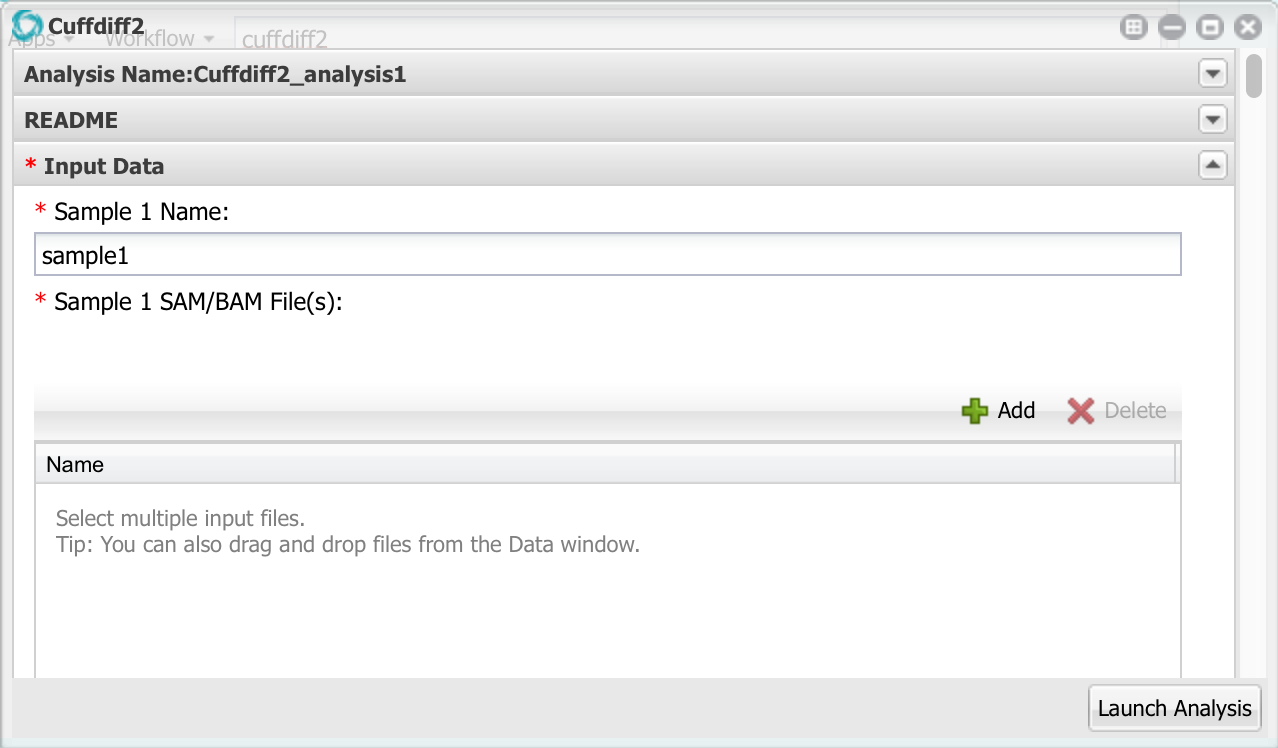
Here we can enter up to 10 different samples, but we only need to use the first two. Change the name of sample 1 to ’24hpi’. Then, click the add button and add the two bam files for the 24 hpi sample. Remember to select the bam files, NOT the FASTQ files!
 Now go down to sample 2 and configure it with the 60hpi bam files.
Scroll down and find the sections for Reference Annotations and Reference Genome. Add the .gtf file to the reference annotations section and the .fasta file to the reference genome section. Remember that these files are in the shared folder named rna-seq-tutorial.
Now you are ready to run cuffdiff. Click the Launch Analysis button. This analysis can take 30 minutes or longer, depending on how busy Discovery Environment is. Go get a cup of coffee.
Step 3: Examine the cuffdiff reports.
Click on the Analysis name in the Analysis window to open the results. Inside you will see several reports. The most important ones are in the folder cuffdiff_out. Open that folder.
Inside you will see several files. For this tutorial we will focus on the file gene_exp.diff. We will download this file and open it in LibreOffice or Excel. To download it, select it, and then select Download -> Simple Download… from the menu:

Open this file as a spreadsheet with LibreOffice or with Excel.
In LibreOffice, select File -> Spreadsheet. Then, select File -> Open. Navigate to the gene_exp.diff file and open it.
You will see several columns of numbers. The most important ones are value_1 and value_2 columns which contain the FPKM values for the 24hpi and 60hpi samples. the second to last column is labeled q_value. The Q value is similar to a P value but it includes a correction for multiple tests. the last column, significant, has a yes or no for each gene to indicate whether or not they are significant.
The data table also contains a column called log2(fold_change) which is log2 of the ratio of the FPKM samples. From the menu in LibreOffice, select Data -> Sort. Sort data data using the column log2(fold_change):
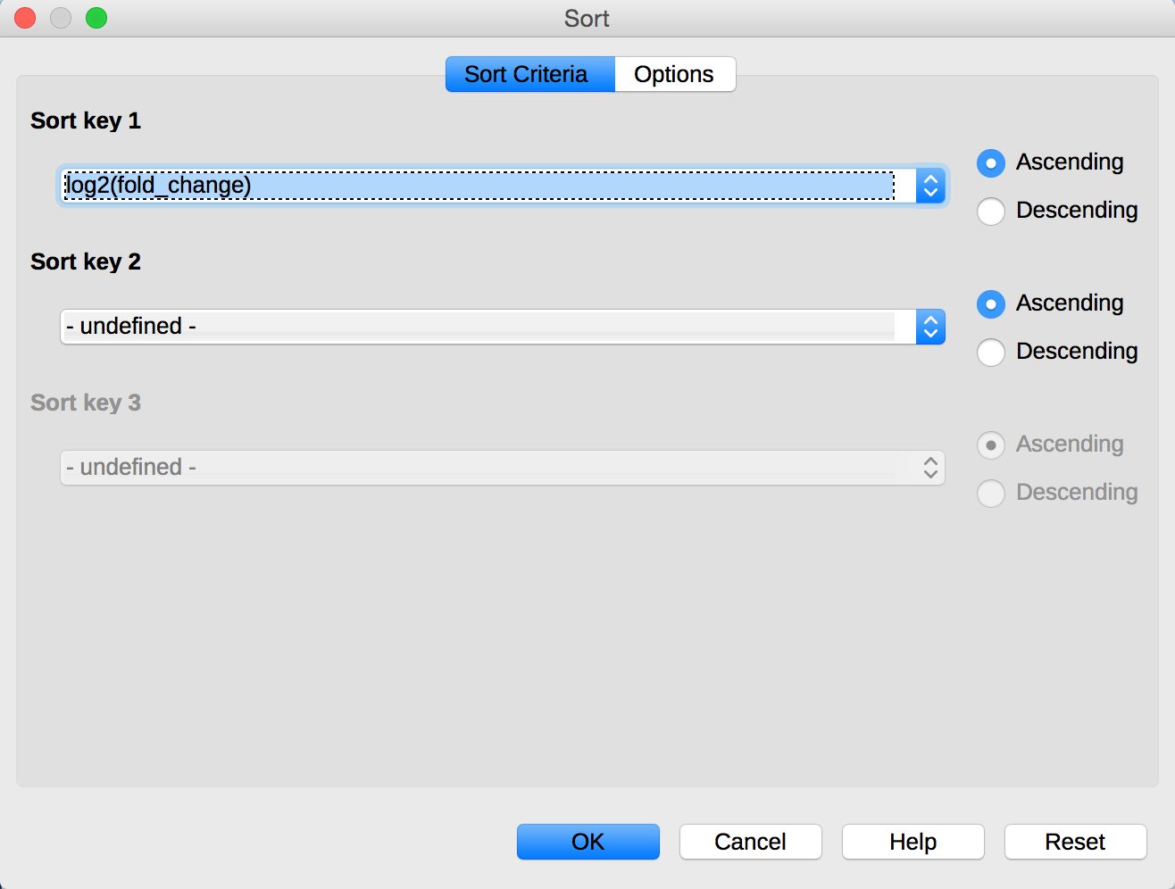
You can see that the table is now sorted by the genes that are most highly expressed in the 24hpi sample compared to the 60hpi sample.
Which gene is most highly expressed in the 24hpi sample compared to the 60hpi sample and that also has a statistically significant difference?
Which gene is most highly expressed in the 60hpi sample compared to the 24hpi sample and that also has a statistically significant difference?
How many genes are expressed in the 24hpi sample but NOT detected in the 60hpi sample?
What are the five genes most upregulated in the 24hpi sample compared to the 60hpi sample?